This notebook computes the curve length using Maxima and Euler. For an example, we start with the logarithmic spiral.
>a=0.1;  ...
   plot2d("exp(a*x)*cos(x)","exp(a*x)*sin(x)",r=2,xmin=0,xmax=2*pi):
>function fx(t) &= exp(a*t)*cos(t)
                              a t
                             E    cos(t)
>function fy(t) &= exp(a*t)*sin(t)
                              a t
                             E    sin(t)
Compute the elements of curve length ds, and simplify the result.
>&sqrt(diff(fx(t),t)^2+diff(fy(t),t)^2), df &= trigreduce(radcan(%))
                a t           a t        2
       sqrt((a E    sin(t) + E    cos(t))
                                           a t           a t        2
                                     + (a E    cos(t) - E    sin(t)) )


                                2       a t
                          sqrt(a  + 1) E
>&df
                                2       a t
                          sqrt(a  + 1) E
And integrate to find the curve length.
>res &= integrate(df,t,0,2*%pi)
                                     2 pi a
                            2       E         1
                      sqrt(a  + 1) (------- - -)
                                       a      a
Now we can compute the length of our spiral.
>res(a=0.1)
8.78817491636
The next example is the parabola.
>plot2d("x^2",xmin=-1,xmax=1,r=1):
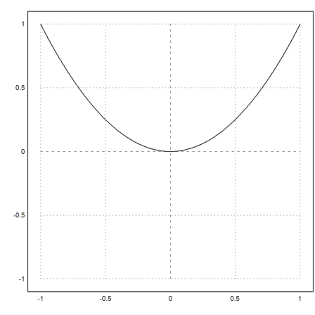
>&integrate(sqrt(1+diff(x^2,x)^2),x,-1,1), %()
                         asinh(2) + 2 sqrt(5)
                         --------------------
                                  2

2.95788571509
Let us compute the length of a line segment with points on the curve.
>x=-1:0.2:1; y=x^2; plot2d(x,y,r=1);  ...
   plot2d(x,y,points=1,style="[]",add=1):
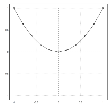
The result is approximately the same as the continuous result.
>i=1:cols(x)-1; sum(sqrt((x[i+1]-x[i])^2+(y[i+1]-y[i])^2))
2.95191957027
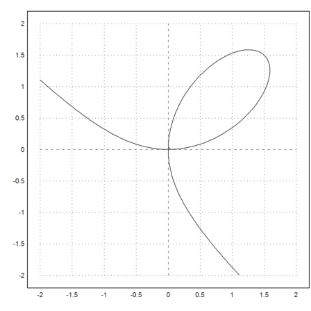
The next example is called the Cartesian curve. It is an implicit function.
>eq &= x^3+y^3-3*x*y
                            3            3
                           y  - 3 x y + x
First, we plot it.
>plot2d(eq,r=2,level=0,n=100):
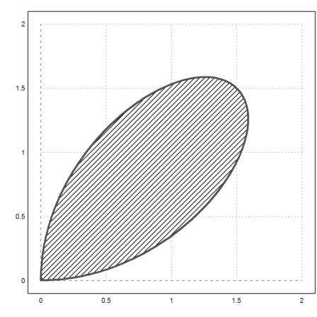
We are interested in the part in the positive quadrant.
>plot2d(eq,a=0,b=2,c=0,d=2,level=[-10;0],n=100,contourwidth=3,style="/"):
We solve it for x.
>&eq with y=l*x, sol &= solve(%,x)
                          3  3    3        2
                         l  x  + x  - 3 l x


                               3 l
                         [x = ------, x = 0]
                               3
                              l  + 1
And define a function in Maxima.
>function f(l) &= rhs(sol[1])
                                 3 l
                                ------
                                 3
                                l  + 1
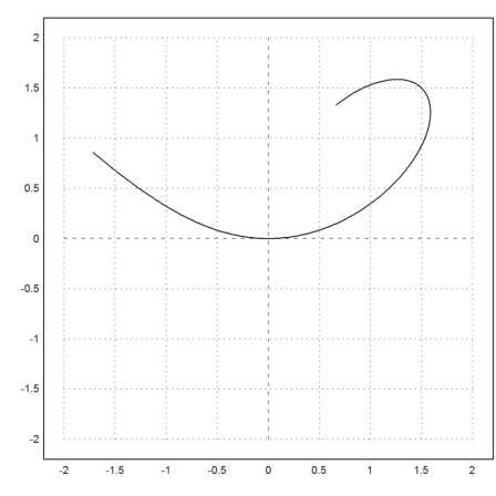
Now we use the function to plot the curve in Euler.
>plot2d(&f(x),&x*f(x),xmin=-0.5,xmax=2,a=0,b=2,c=0,d=2,r=2):
Compute the curve element ds.
>&ratsimp(sqrt(diff(f(l),l)^2+diff(l*f(l),l)^2))
                    8       6       5       3       2
            sqrt(9 l  + 36 l  - 36 l  - 36 l  + 36 l  + 9)
            ----------------------------------------------
                        12      9      6      3
                  sqrt(l   + 4 l  + 6 l  + 4 l  + 1)
Maxima cannot integrate this.
>&integrate(%,l,0,1)
          1
         /          8       6       5       3       2
         [  sqrt(9 l  + 36 l  - 36 l  - 36 l  + 36 l  + 9)
         I  ---------------------------------------------- dl
         ]              12      9      6      3
         /        sqrt(l   + 4 l  + 6 l  + 4 l  + 1)
          0
So we use fast numerical integration in Euler. To get the part in the first quadrant, we integrate from 0 to 1, and double the result.
>2*romberg(&(sqrt(diff(f(x),x)^2+diff(x*f(x),x)^2)),0,1)
4.91748872168
We can put the computation of the curve length into a function in Euler. The function will use Maxima each time it is called to compute the derivative.
>function curvelength (fx,fy,a,b) ...
 ds=mxm("sqrt(diff(@fx,x)^2+diff(@fy,x)^2)");
 return romberg(ds,a,b);
 endfunction
>curvelength("x","x^2",-1,1)
2.95788571509
>2*curvelength(mxm("f(x)"),mxm("x*f(x)"),0,1)
4.91748872168
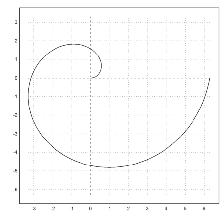
Finally the Archimedean spiral.
>curvelength("x*cos(x)","x*sin(x)",0,2*pi)
21.2562941482
>plot2d("x*cos(x)","x*sin(x)",xmin=0,xmax=2*pi,square=1):
The following function computes the line element for given expressions fx and fy in Maxima only.
>function ds(fx,fy) &&= sqrt(diff(fx,x)^2+diff(fy,x)^2)
                           2              2
                  sqrt(diff (fy, x) + diff (fx, x))
>sol &= ds(x*cos(x),x*sin(x))
                                  2                      2
          sqrt((cos(x) - x sin(x))  + (sin(x) + x cos(x)) )
>&sol | trigreduce | expand, &integrate(%,x,0,2*pi), %()
                                   2
                             sqrt(x  + 1)


                                              2
                  asinh(2 pi) + 2 pi sqrt(4 pi  + 1)
                  ----------------------------------
                                  2

21.2562941482
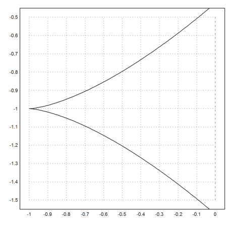
Another example.
>sol &= radcan(ds(3*x^2-1,3*x^3-1))
                                      2
                          3 x sqrt(9 x  + 4)
>plot2d("3*x^2-1","3*x^3-1",xmin=-1/sqrt(3),xmax=1/sqrt(3),square=1):
>&integrate(sol,x)
                                2     3/2
                            (9 x  + 4)
                            -------------
                                  9
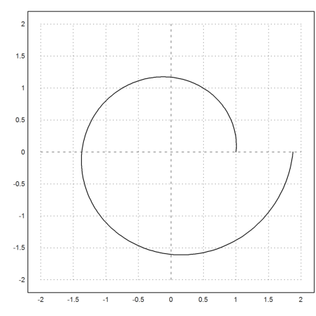
We compute the length of the curve defined by a point on a rolling wheel. The wheel is rolling to the left, so that its center is in
![]()
at time t. The wheel has radius 1 for simplicity, so that it has turned to the left once if t=2*pi. The point, where the wheel touches the ground at time t=0 follows the curve
![]()
To check this, set t=0. Then observe that (sin(t),cos(t)) does indeed turn to the left.
>ex &= x-sin(x); ey &= 1-cos(x);
We plot the curve and the state of the wheel at t=2.
>plot2d(ex,ey,xmin=0,xmax=2pi,square=1); ...
   plot2d("2+cos(x)","1+sin(x)",xmin=0,xmax=2pi,>add,color=red); ...
   plot2d([2,ex(2)],[1,ey(2)],color=red,>add); ...
   plot2d(ex(2),ey(2),>points,>add,color=red):
>&sqrt(diff(x-sin(x),x)^2+diff(1-cos(x),x)^2) | radcan, f &= trigsimp(%)
                        2         2
                sqrt(sin (x) + cos (x) - 2 cos(x) + 1)


                          sqrt(2 - 2 cos(x))
>&integrate(f,x,0,2*pi)
8
Of course, numerical integration works too.
>romberg(mxm("f"),0,2*pi)
8
Now we use Maxima to compute the curvature, and the evolute of curves.
First, we define a function for the curve segment ds of a curve f(t) = [fx(t),fy(t)] in Maxima.
![]()
It is the norm of the derivative vector, or speaking in terms of physics, the speed at the time t.
>function dsf(fx,fy,t) &&= sqrt(diff(fx,t)^2+diff(fy,t)^2)
                           2              2
                  sqrt(diff (fy, t) + diff (fx, t))
Of course, this is the length of the circumference for a circle, if we take one turn in one second.
>&assume(r>0); &trigsimp(dsf(r*cos(2*pi*x),r*sin(2*pi*x),x))
2 pi r
The length of the curve is the integral over the speed. This is obvious in physics. With the right definition for the curve length, it can be proved exactly.
![]()
Let us compute the length of the parabola from -1 to 1.
>&integrate(dsf(x,x^2,x),x,-1,1), %()
                         asinh(2) + 2 sqrt(5)
                         --------------------
                                  2

2.95788571509
We can check this numerically in Euler. We add the lengths of curve segments for this.
>t=-1:0.01:1; s=t^2; n=cols(t);  ...
   sum(sqrt((differences(t))^2+(differences(s))^2))
2.95787080795
Now, we setup a function for the curvature of a curve [fx,fy]. We can only motivate the formula. The vector
![]()
is perpendicular to f'(t) with the same length. Thus the scalar product
![]()
is the part of the acceleration perpendicular to the path times the speed. Let us compute this for a general path along a circle with constant speed.
>gx &= r*cos(om*t); gy &= r*sin(om*t); ...
    &trigsimp(diff(gx,t)*diff(gy,t,2)-diff(gy,t)*diff(gx,t,2))
                                  3  2
                                om  r
The speed is the following.
>&assume(om>0); &trigsimp(dsf(gx,gy,t))
om r
If we divide the speed to the third power by the expression above, we get the radius for this specific case.
![]()
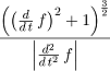
We take this as a definition of curvature for general curves, since we can assume the acceleration and the speed to be asymptotically constant locally.
>function kr(fx,fy,t) &&=  dsf(fx,fy,t)^3 ...
   /abs(diff(fx,t)*diff(fy,t,2)-diff(fx,t,2)*diff(fy,t))
                                  3
                               dsf (fx, fy, t)
        -------------------------------------------------------------
        mabs(diff(fx, t) diff(fy, t, 2) - diff(fx, t, 2) diff(fy, t))
Let us check with a circle of radius r.
>&assume(r>0); &trigsimp(kr(r*cos(om*x),r*sin(om*x),x))
r
We get the well known formula for the curvature of the parabola.
>&ratsimp(kr(t,t^2,t))
                                2     3/2
                            (4 t  + 1)
                            -------------
                                  2
The general formula for the curvature of the graph of a function
![]()
it the following.
>&remvalue(f); &depends(f,t); $kr(t,f,t)
Now we want to compute the center of the curvature at any point [fx,fy] depending on t. Again, we cannot provide an explanation for the formula here.
The following factor is common to both coordinates.
>function kra(fx,fy,t) &&=  dsf(fx,fy,t)^2 ...
   /(diff(fx,t)*diff(fy,t,2)-diff(fx,t,2)*diff(fy,t))
                               2
                            dsf (fx, fy, t)
        -------------------------------------------------------
        diff(fx, t) diff(fy, t, 2) - diff(fx, t, 2) diff(fy, t)
Now the x and y coordinates depending on x.
>function ux(fx,fy,t) &&= fx-diff(fy,t)*kra(fx,fy,t)
fx - kra(fx, fy, t) diff(fy, t)
>function uy(fx,fy,t) &&= fy+diff(fx,t)*kra(fx,fy,t)
fy + kra(fx, fy, t) diff(fx, t)
Combine to a curve.
>function krm(fx,fy,t) &&= [ux(fx,fy,t),uy(fx,fy,t)]
[ux(fx, fy, t), uy(fx, fy, t)]
Let us test with the circle of radius r.
>&trigsimp(krm(r*cos(x),r*sin(x),x))
[0, 0]
For the parabola, we get a special curve.
>&ratsimp(krm(x,x^2,x))
                                      2
                                3  6 x  + 1
                          [- 4 x , --------]
                                      2
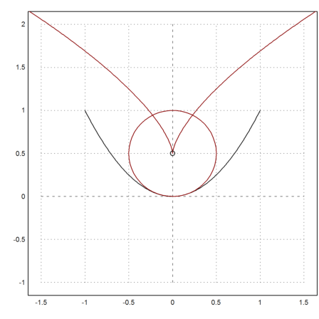
Let us plot this in Euler. First the parabola.
>plot2d("x","x^2",xmin=-1,xmax=1,a=-1.5,b=1.5,c=-1,d=2);
Then add the curve of the midpoints.
>plot2d(mxm("ux(x,x^2,x)"),mxm("uy(x,x^2,x)"),xmin=-1,xmax=1,color=2,add=1);
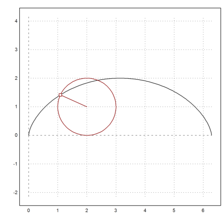
Now compute the radius and the center at a specific point.
>xt=0; m=mxmeval("krm(x,x^2,x)",x:=xt); r=mxmeval("kr(x,x^2,x)",x:=xt); ...
 plot2d("m[1]+cos(x)*r","m[2]+sin(x)*r",xmin=0,xmax=2*pi,add=1,color=2); ...
 plot2d(m[1],m[2],points=1,style="o",add=1):
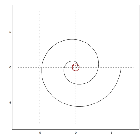
Next, let us investigate the logarithmic spiral.
>a=1; k=0.15; plot2d("a*exp(k*x)*cos(x)","a*exp(k*x)*sin(x)", ...
   xmin=-4*pi,xmax=4*pi,r=7,n=500):
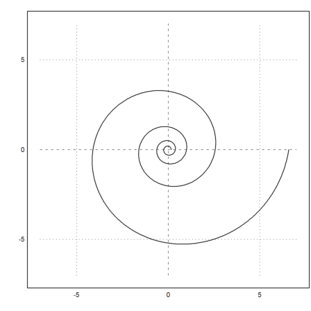
To see everything, we need a less complicated plot.
>a=1; k=0.15;
>plot2d("a*exp(k*x)*cos(x)","a*exp(k*x)*sin(x)",xmin=0,xmax=2*pi,r=3,n=500);
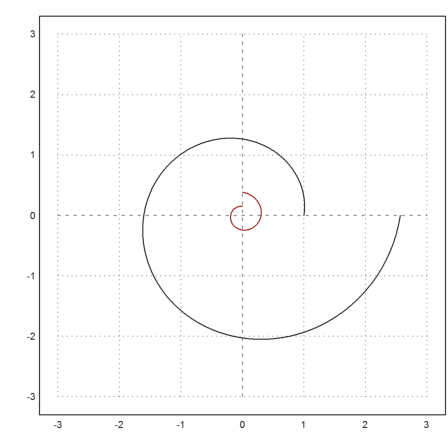
Let us compute the centers of curvature.
>&assume(a>0); &ratsimp(krm(a*exp(k*t)*cos(t),a*exp(k*t)*sin(t),t))
                         k t              k t
                 [- a k E    sin(t), a k E    cos(t)]
This is again a logarithmic spiral. We add it to the plot.
>plot2d("-a*k*exp(k*x)*sin(x)","a*k*exp(k*x)*cos(x)", ...
   color=2,xmin=0,xmax=2*pi,add=1,n=500):
What about the Archimedean spiral?
>a=2; plot2d("x*cos(a*x)","x*sin(a*x)",xmin=0,xmax=2*pi,r=8,n=500);
This spiral adds the same amount to the radius at each winding. Let us compute the centers of curvature.
>&assume(a>0); &ratsimp(krm(x*cos(a*x),x*sin(a*x),x))
                          2  2
         a x cos(a x) - (a  x  + 1) sin(a x)
        [-----------------------------------,
                      3  2
                     a  x  + 2 a
                                                   2  2
                                  a x sin(a x) + (a  x  + 1) cos(a x)
                                  -----------------------------------]
                                               3  2
                                              a  x  + 2 a
And add to the plot. We see that the curve converges to a circle.
>plot2d(mxm("ux(x*cos(a*x),x*sin(a*x),x)"), ...
   mxm("uy(x*cos(a*x),x*sin(a*x),x)"),xmin=0,xmax=2*pi,add=1,color=2):